
Sulphur 404 Jan-Feb 2023

31 January 2023
Sulphur run-down liquid level prediction
SULHUR HANDLING
Sulphur run-down liquid level prediction
Sulphur run-down lines are typically sized by referencing past projects and ‘rules of thumb’. Very little analysis is performed to identify the impacts of slope, fittings, valves, etc. It is critical to maintain an open vapour path from the condenser to the sealing device. CSI has observed problems in the field which appear to be caused by undersized run-down lines. CSI developed a method of predicting the liquid level in a run-down line that considers the most common elements. This was accomplished by building a full-scale model of a run-down line that evaluated pipe NPS, pipe slope, rod-out-cross elbows, rod-out cross elevation drops, and liquid viscosity. This article presents the testing and development of the predictive method as well as the predictive method itself.
In a Claus sulphur recovery unit, sulphur is continuously produced in a series of condensers (typically four per train). These condensers operate at an elevated pressure (typically 1 to 8 psig/0.07 to 0.55 bar). The sulphur is continuously drained from the condensers via the rundown lines. These lines run from the condenser drain to a sealing device, and from the sealing device to a sulphur storage container. It is critical that the process gas remains in the condensers so it can continue through for further processing. The sealing device is a passive device that allows the sulphur to pass through, while preventing vapour from escaping. The sealing device operation is comparable to the function of a steam trap.
Flow in a sulphur run-down is effectively ‘open channel’ flow. It is critical that these lines have open channel flow for three reasons:
- Having a continuous downward slope ensures that the lines will drain. This is convenient for maintenance operations, and, more importantly, avoids the accumulation of debris at low points resulting in obstruction. Open channel flow results.
- Sulphur accumulation in the condenser is to be avoided. The run-down lines must be sized for something greater than the maximum production rate. Open channel flow results.
- Vapour displaced from the sulphur sealing device must have an open path to the condenser to prevent vapour locking. The vapour space of the sealing device must operate at the same pressure as the condenser and a vapour path from the sealing device to the condenser must be maintained to ensure this. Note that this is true of all popular sealing devices including traditional seal legs, SulTraps manufactured by SOS, and SxSeals manufactured by CSI.
The sulphur industry typically sizes run-down lines based on rules of thumb, past experience, and occasional theoretical calculations performed by engineering companies. No best practice approach exists for either the philosophy (vapour path opening size, debris accumulation safety factor) or for the method. The industry would benefit from a more rigorously developed approach.
Approach
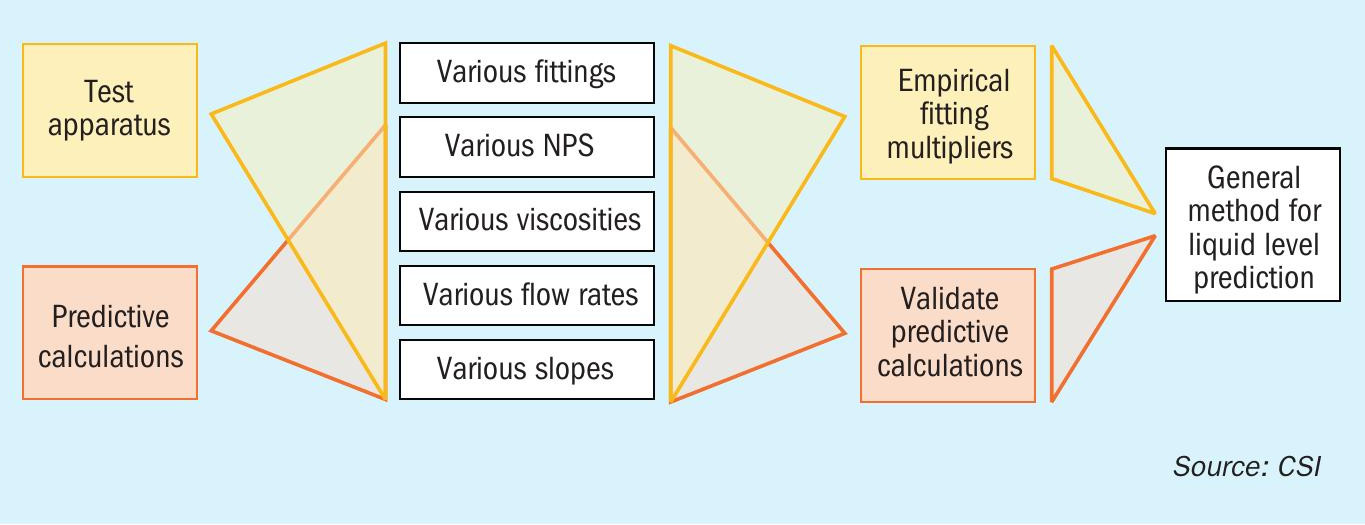
CSI’s goal was to develop a general method of predicting the liquid level and maximum capacity of sulphur run-down lines. This was accomplished using a combination of predictive calculations and physical testing. Predictive calculations can be applied to steady, open channel flow in a straight run, but predictive calculation is difficult when applied to flow through fittings and transitional regions. The work performed to develop the general method consisted of:
- development of a predictive calculation method for straight runs;
- assembly of a full-scale model of a rundown line incorporating common elements;
- testing with water of varying viscosity from which sulphur flow predictions could be extrapolated;
- validation of the predictive calculations for the straight runs;
- identification of empirical ‘multipliers’ that predict the liquid level in the fittings and transition regions.
Fig. 1 shows a visualisation of the development approach. Much of the work was performed by a five-person team of University of North Carolina, Charlotte undergrad students as their senior design project. The team designed and assembled the apparatus, conducted the test runs, and gathered the data. The team also performed some data analysis, though the final data analysis was performed by CSI engineering.
Test apparatus
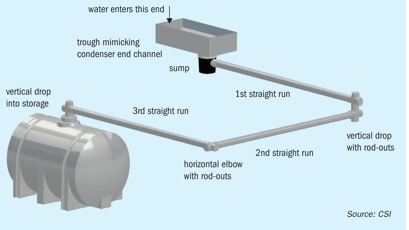
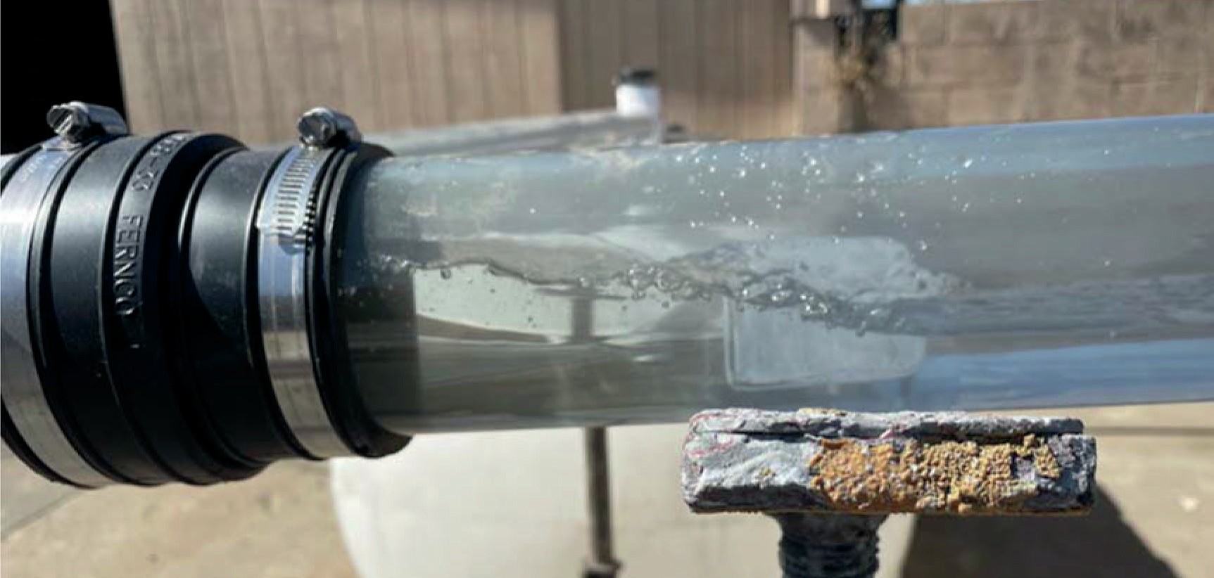
The test apparatus was a full-scale rundown line configurable to evaluate the various items of interest. The material used was primarily clear PVC which enabled measurement of the liquid level within. The test apparatus was configurable to include the following:
- pipe sizes ranging from 2 inches to 4 inches NPS;
- a straight section sufficiently long to produce fully-developed flow;
- various pipe slopes from1/8 in/ft to5/8 in/ft; an entrance region representing a typical sump-style condenser connection;
- a vertical drop made with rod-out crosses;
- a horizontal 90° elbow made with a rod-out cross;
- an exit region representing a vertical drop into a sulphur pit.
The use of clear PVC prevented testing with sulphur. Instead, thickened water was used to mimic the flow characteristics of sulphur. Thus, the fluid conditions that could be evaluated included:
- water at various viscosities;
- various flow rates.
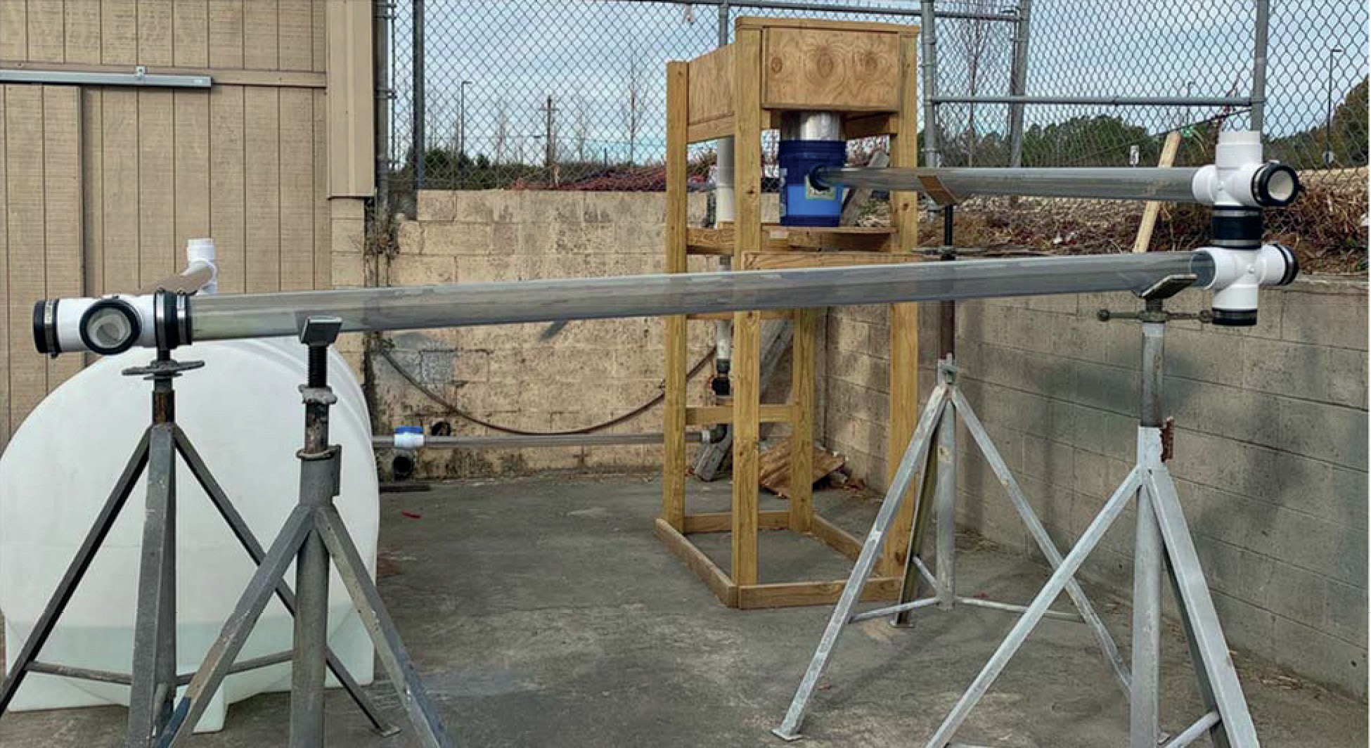
Fig. 2 shows the test apparatus layout.
Without the ability to test sulphur directly, it was necessary to manipulate the water viscosity to mimic the flow characteristics of sulphur. Reynolds number is strongly predictive of flow characteristics. Thus, the target water viscosities were based on achieving the same Reynolds number in testing as will be seen in sulphur. Specifically, the same density/dynamic viscosity ratio (rho/mu).
Sulphur’s viscosity increases dramatically above 318°F (159°C) when the sulphur molecules form polymer chains. The presence of H2S in the sulphur has the effect of capping those chains and reducing the sulphur viscosity. As a high-end viscosity, CSI considered a first condenser condition of 350°F (177°C), 500 ppm H2S, and 50 cP. At the low end, CSI considered a fourth condenser condition of 280°F (138°C), 25 ppm H2S, and 9 cP. These viscosities were arrived at using work published by ASRL (Rheometric Properties of Liquid Elemental Sulphur and Modifying Effects of Hydrogen Sulphide; Alberta Sulphur Research Ltd. 2019). CSI conducted testing across a larger viscosity range to extend the applicability of the results. A water viscosity range of 1 to 36 cSt was tested, which is equivalent to a sulphur viscosity range of 3 to 115 cP. A total of 91 test runs were conducted.
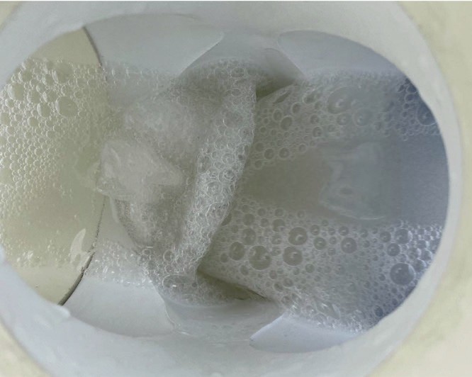
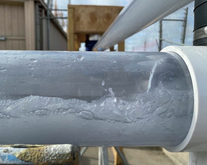
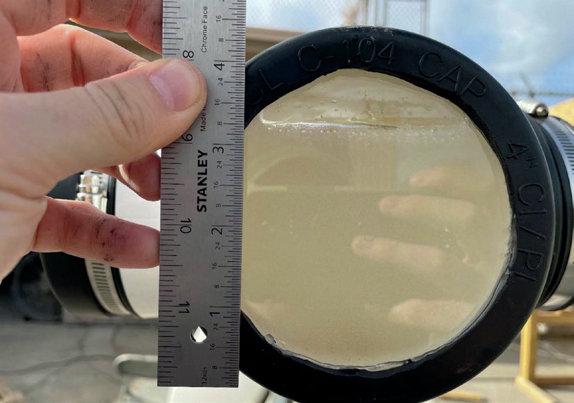
The test apparatus provided control of the inputs: pipe NPS, pipe slope, fluid flow rate, fluid viscosity, and fitting configuration. The primary measured parameter was the liquid level at various locations along the line. At ten locations holes were drilled in the top of the pipe and a depth gauge was used to measure the liquid level. Additionally, a clear window was installed on each ‘blind’ of the rod-out fittings; this was used to observe the flow characteristics and to measure the liquid level against the window (see photos).
Uncertainty
Through the course of testing and analysis, three areas of uncertainty were identified. These are unlikely to have a significant impact on the conclusions of the study but need to be acknowledged.
Inconsistent slope: For the majority of the test runs, the slope was measured referencing the concrete slab on which the apparatus was assembled. This was later identified as a source of significant error as the slab was not level. The tests were not re-run, rather the slope data was corrected for the analysis. As a result, for each test run, each of the three pipe runs in the test apparatus was set to a different slope. This differed from the intended test setup and may have introduced some amount of error as each of the fittings had a slightly different slope entering vs exiting the fitting.
Fully developed flow: The straight run pipe lengths were chosen to ensure fully developed flow. This analysis was based on L/D recommendations for internal flow. But during testing it was observed that the open channel would form standing waves and other flow variability that extended for the full length of the pipe. The pipe lengths were not sufficient to ensure fully developed flow. The impact of this was most significant in the first straight run as discussed in the next point.
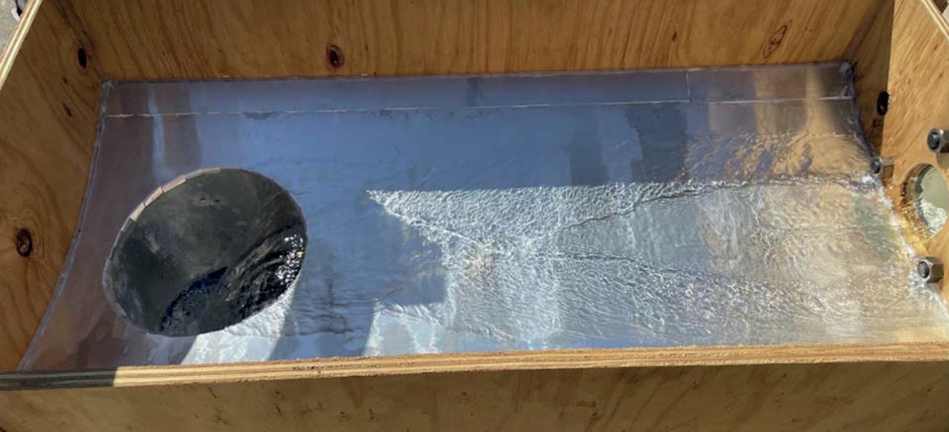
Sump region flow pattern: The first section of the test setup was intended to mimic a sump on the bottom of a sulphur condenser. In a sulphur condenser the sulphur waterfalls down the tubesheet and forms a river of sulphur in the ends channel heading towards the sump. It is speculated that this ‘river’ has relatively even flow distribution. But in the test setup, the water was delivered to the ‘end channel’ via a pipe. The flow of water discharging from the pipe created currents and standing waves in the end channel and sump that carried through to the run-down line. To mitigate this, baffles were inserted in front of the pipe discharge to create a more even distribution of flow entering the sump. This successfully eliminated the standing waves and other flow variations in the first straight pipe. But the original intention of accurately representing the condenser sump was not achieved.
Predictive calculations
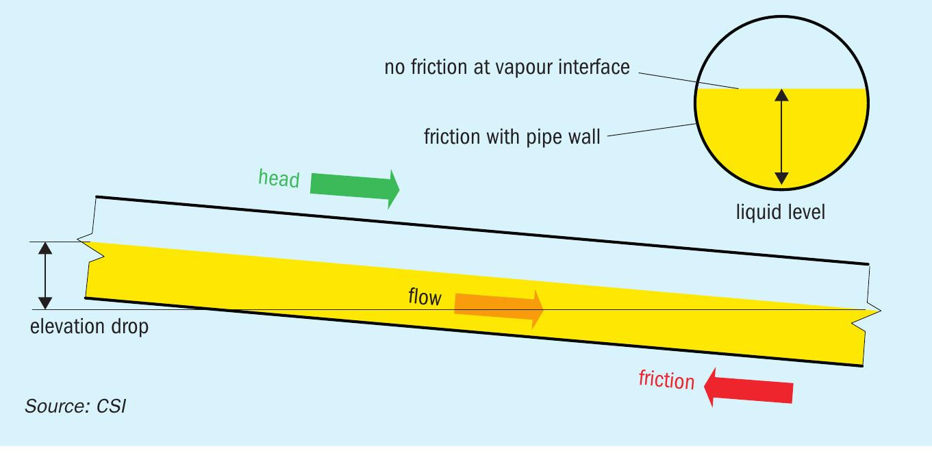
For steady-state conditions in straight pipe, the liquid level can be predicted using fluid theory (Fig. 3). At steady state, the energy of the system balances. In the case of gravity-driven flow, the two energy paths in balance are energy loss due to friction with the pipe wall, and energy gain due to elevation drop (liquid head).
The liquid head is calculated as elevation drop per unit length of pipe. The frictional loss is calculated using the Darcy-Weisbach equation with modification to consider the partial cross-section of the fluid in the pipe. Specifically, the liquid-vapour interface surface is considered to have no frictional losses and is therefore omitted from the calculation.
The conventional presentation of Darcy’s equation is re-arranged to solve for the pipe slope:
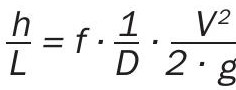 where:
h = elevation drop per unit length
L = unit length of pipe
f = pipe wall friction factor calculated from Reynolds number where Reynolds number uses the fluid hydraulic diameter D
D = fluid hydraulic diameter = 4* (liquid cross section)/(liquid arc length contacting the pipe wall)
V = fluid velocity
g = gravity constant
CSI’s approach was to consider a fixed slope and flow rate; then to find the liquid level by iteration. f, D, and V on the right side of the equation are all functions of liquid level and change with each iteration. The liquid level is iterated until both sides of Darcy’s equation balance. This approach is valid for straight pipe with a constant slope and fully developed flow.
CSI did not attempt to predict the liquid level in the fittings, choosing instead to depend empirically on the test results. It is likely that modelling the liquid level in the fittings would require sophisticated CFD modelling. This was beyond the capabilities of the group working on the project.
Test results
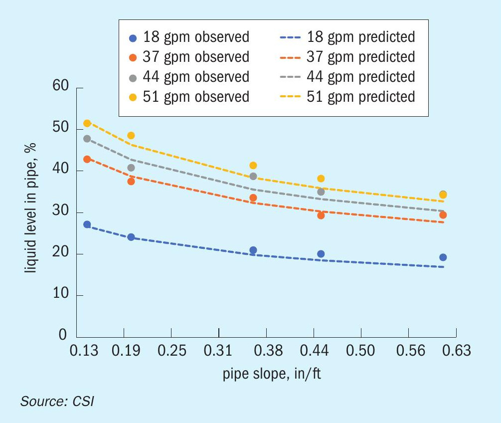
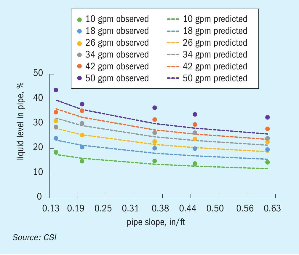
The test results for straight pipe all trend as expected. Pipe NPS, fluid viscosity, fluid flow rate, and pipe slope all have the expected effect on the liquid level. Overall, the formula tends to slightly under-predict the liquid level. The under-prediction is minor for most of the tested range, becoming significant only for lower viscosities running at higher flow rates. The graphs in Figs 4 and 5 show this comparison for 4-inch NPS pipe at two different viscosities. Points are observed data; dotted lines are the prediction. The other NPS/viscosity combinations follow the same trends.
The test points shown in the graphs in Figs 4 and 5 are all below the 50% liquid level. This is because the liquid level in the fittings was roughly 2x higher than the liquid level in the straight pipe. The test flow rate was limited by the fittings. This is expected as the fluid tends to slow down and ‘pile up’ in the fitting before it changes direction and starts flowing again. Interestingly, the liquid level observed in the fittings is higher than one would expect based solely on conservation of energy (Bernoulli’s equation). This indicates that fluid momentum creates highly dynamic flow conditions in the fittings. Indeed, the liquid movement in the fittings was considerably more turbulent than in the straight runs.
The liquid in the fittings would slosh around and bounce up and down making it difficult to determine the true liquid level. Liquid level measurements were taken at the fittings with the intention of capturing the average liquid level; it is felt that this was accomplished reasonably well. Even though the data has a lot of scatter, the trends of the averages still follow a logical pattern.
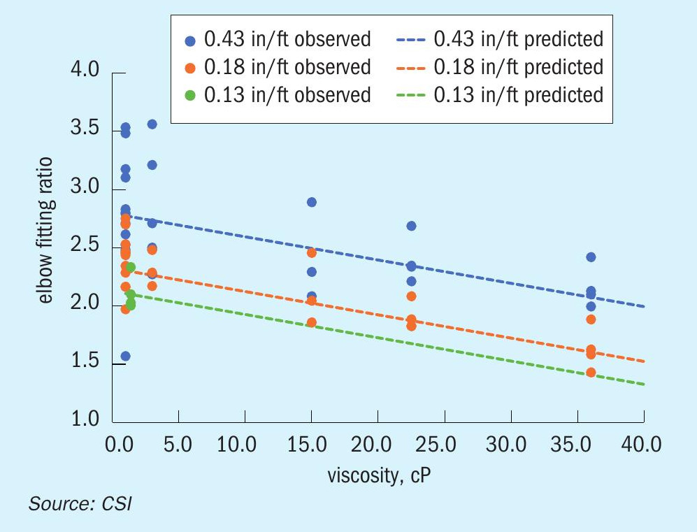
To analyse the fitting data, the observed fitting liquid level was divided by the predicted straight pipe liquid level to product a ‘fitting ratio’. It was found that the fitting ratio was dependent on the fluid viscosity and the pipe slope, but not on the fluid flow rate or the pipe NPS. Formulas for the fitting ratios were developed from the data.
Horizontal rod-out elbow:
Ratio = (-0.02) * viscosity + 0.54 * ln(slope) + 3.25
where viscosity units are cP and slope units are in/ft
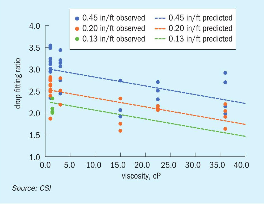
Vertical drop elbow:
Ratio = (-0.02) * viscosity + 0.59 * ln(slope) + 3.49
where viscosity units are cP and slope units are in/ft
The vertical drop tended to produce a slightly larger liquid level. This is reflected in the last term of the two formulas. The charts in Figs 6 and 7 show the observed fitting ratios compared to those predicted by the formula.
A similar analysis was conducted for the sump nozzle. It was expected that the transition from low velocity in the sump to higher velocity in the pipe would result in liquid level drop as energy is conserved. This was observed, but the data was very scattered, and trends were difficult to establish. This was likely due to the inconsistent flow characteristics in this region as previously discussed. A fitting ratio formula was derived from the data, but its accuracy is questionable considering the uncertainty surrounding this area of the test.
Ratio = 0.98 * slope + 1.04
where slope units are in/ft
The test setup also included a vertical drop into the collection vessel mimicking a typical discharge into a sulphur pit. As expected, there was never any backup of liquid in this region; a clear vapour path was always present in all test runs.
Application
The test data and analysis provided formulas that can be used to predict the liquid level in sulphur rundown lines of various configurations. In theory, when the liquid level reaches 100% at any point in the line, vapour can no longer exchange between the sulphur condenser and the sealing device, and a vapour lock scenario becomes possible. This should provide an engineer with the ability to determine the maximum liquid capacity of a given line. But the real-world application is a bit fuzzier. The following factors should also be considered by any engineer endeavouring to apply these findings:
Sloshing vapour exchange: The test did not directly evaluate the ability of vapour to travel through the line. From the observations, it is speculated that even when the fitting liquid level is at 100%, the ‘sloshing’ of the fluid in the line opens intermittent vapour paths that are sufficient for pressure equalisation under normal conditions. This is an argument for more aggressive line sizing.
Debris accumulation: Accumulation of debris in the form of tar-like material build-up on the pipe walls is relatively common in SRUs. This accumulation effectively reduces the cross-section of the pipe resulting in diminishing capacity over time. This is an argument for more conservative line sizing.
Valve design: Industry best practice is to use full-port plug or ball valves in rundown lines; these should have minimal effect on the fluid level in the pipe. But other valves are often encountered; any reduction in the line cross-section will create a restriction point. This is an argument for more conservative line sizing when valve choice is sub-optimal.
Fitting frequency: The test was constructed to evaluate the fittings in isolation. A series of fittings in close succession would result in slower fluid velocity and a higher liquid level in the pipe. This is an argument for more conservative line sizing when fittings density is high.
Varying slope: The test was conducted with relatively consistent slope throughout. Many real-world applications have multiple section of pipe with varying slope. This is acceptable provided the calculations are based on the shallowest slope. But many run-down lines include short sections of near-level pipe. This is an argument for more conservative line sizing when there are near-level sections of pipe.
Experience: CSI has observed several running plants that appear to be operating without issue despite having run-down lines that would be considered under-sized based on this test data. It is speculated that, in most real-world applications, intermittent vapour exchange provides sufficient pressure equalisation between the sulphur condenser and the sealing device. This is an argument for more aggressive line sizing.
Summary
A series of test was conducted to characterise the liquid level in run-down line piping. The purpose was to establish a method of sizing these lines to ensure proper vapour pressure equalisation between the sulphur condenser and the sealing device. The tests considered many of the common elements of a rundown line. The results led to the development of a set of formulas that can be applied to a variety of rundown line configurations to predict the liquid level. The formulas should not be applied blindly as there are several over factors to consider when sizing run-down lines. These factors are briefly discussed and require engineering judgement for their application.
The authors of this article are Brandon Forbes of Ametek/Controls Southeast and the University of North Carolina Charlotte Senior Design Team – Joseph Tucker, Armias Adhanom, Justin Domingo, Baron Le and Reagan Rushing.